Machine learning provides an excellent avenue for predicting future energy consumption.
Energy Consumption is Ripe for ML Predictions
Matching energy consumption with the appropriate level of supply is critical. Excess electricity cannot be stored unless converted to alternate forms, which invokes additional resources and costs. Underestimating energy consumption can be highly detrimental, with demand overloading supply lines and causing blackouts. There are tangible benefits to monitoring and anticipating consumption trends across residential and commercial applications.
Machine learning provides an excellent avenue for predicting future energy consumption. Accurate insights can provide critical insights into variables affecting demand, providing decision-makers with an opportunity to address these levers. Forecasts also provide a benchmark to identify anomalous behavior, either high/low consumption, and alert managers to faults within the building.
Firms are investing significant effort into finding creative ways of applying machine learning (ML) and artificial intelligence (AI) to accurately forecast energy consumption, especially with the rise of renewable sources.
Mosaic Data Science sees several ML-driven improvements that can help distributors better anticipate consumption needs and deploy probabilistic electricity consumption forecasting.
Improving Smart Meter Forecasts with Machine Learning
Forecasts of future events based on careful modeling and analysis of the past are ubiquitous in the business environment. Traditionally, these forecasts are derived from a class of algorithms known as “deterministic” models. Whether a complex statistical model or a black-box deep learning application, deterministic models formalize a direct map from an input to an expected output. In other words, given the same input values, the output value will not change once the model is established. These output values are known as point estimates.
Although well accepted and used to significant effect, estimates often represent the outcome value that can be expected “on average” for the given inputs. This phenomenon suggests that many plausible outcomes may be higher or lower for any provided point estimate than the predicted value.
When making decisions that affect personnel, profit or investment in future growth, it is advantageous to have more than just a “point estimate” at hand. In these scenarios, we can instead use “probabilistic” models to capture and express uncertainty around the outcomes and the various inputs contributing to the estimates.
For this article’s purposes, we will specifically explore the application of a class of probabilistic models known as Dynamic Linear Models (DLM). These models are particularly well suited for forecasting time series. Unlike black-box applications, they provide additional and direct insight into the elements that compose the forecast.
Without going into too much technical detail, DLMs are a type of state-space model. The time series to be modeled is a composite of the various contributing “states,” such as the underlying trend, various seasonality, possible regression variables and the error. The model then learns these states, and more importantly, how they may change over time. It projects from these learned states into the future to make forecasts. The model’s probabilistic nature means that every component is captured and expressed with uncertainty, and this uncertainty is carried through into the estimates. We will explore several different applications of this approach in order to highlight its advantages over traditional point forecasts.1
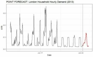
Figure 1: Example of a Point Forecast. Hourly consumption for a London household.
Figure 1 provides an example of a point forecast. In contrast, a probabilistic forecast will convey the average expected value and a range of potential plausible values. A simplified explanation of how the model generates these ranges is that it simulates many possible scenarios and collects these simulations’ results as the forecast distribution.
Figure 2 shows the same forecast as in Figure 1 but presents the range of simulated outcomes at each hour. More specifically, 95% of the results fell within the lighter blue range. In comparison, 70% of the outcomes fell within the darker blue range, and the red line represents the point forecast for the average simulated consumption. The point forecast does pick up on the recent change in consumption patterns, but it fails to express overall historical consumption variability. Incorporating the full range of possible future consumption values allows us to have a more informed, more flexible forecast.
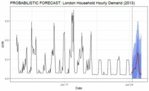
Figure 2: Example of a Probabilistic Forecast. Hourly consumption for a London household.
For this example, we estimate that actual future consumption has a 70% chance of falling between .15 and .6 kWh at its forecast peak. However, we cannot rule out the fact that higher values would not be unexpected. Decisions made solely from the point forecast will not consider any of this legitimate uncertainty and variability. Whether automated or manual, we express uncertainty because a component of the projection can change the very nature in which decisions in an organization are made.
Figure 3: Probabilistic hourly consumption forecast and actuals for a London household.
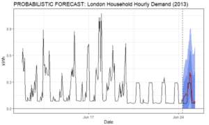
Figure 3: Probabilistic hourly consumption forecast and actuals for a London household.
Figure 3 shows the household’s actual consumption for the forecast period—the new pattern continued uninterrupted.
Although the forecasts here are univariate, they can be significantly enhanced by using additional regressors such as weather data, holidays, and whatever other available information may have a relationship with electricity consumption. Further, although we work with only a few single households here to highlight variety, these techniques can be scaled in multiple ways. They work equally well on fully aggregate data, or cloud-based platforms can be leveraged to build individual models for as many unique time series as desired. Figure 4 shows forecasts for five additional households from a larger batch run with parallel processing.
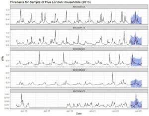
Figure 4: Hourly consumption forecasts and actuals for five London households.
Detecting Residential Consumption Patterns
Consumption patterns vary between consumers, both within a sector such as the residential households we are working with and between sectors such as residential and commercial. Dynamic Linear Models (DLMs) also can provide insight into the elements that contribute to the forecast’s underlying patterns.

Figure 5: Estimated Time-of-Day Adjustments from Baseline for Two Households.
Every consumer has a “baseline” level of electricity consumption, from which actual consumption will vary depending on the time of day, day of the week, weather and other considerations. Figure 5 shows the estimated hour-of-day adjustments from the baseline for two different households over the period in question.
Although the details are more technical than the level of our discussion here, the general conclusions are that these households have relatively different consumption patterns throughout the day. The blue household shows minor variation from its baseline, suggesting less variation overall throughout the day. It also appears that the lower consumption hours for the blue household are shifted forward relative to the green household. Although this example is for hour-of-day patterns, the same breakdown can be applied to any contributing factor, including larger seasonal patterns. Once identified, these patterns can provide additional leverage for activities such as targeted customer communication or service.
Utilities can use sophisticated models such asthe DLMs explored here to not only accurately forecast consumption on micro-and macro-levels, but to do so in a manner that allows for managers to account for the uncertainty inherent in any complex system. These advanced techniques provide a complete picture of consumption drivers by isolating the effects of multiple relevant variables over time. Such insight can enhance other progressive analytics goals, such as clustering consumers for targeted initiative outreach; it also can provide earlier identification of changes in consumption patterns at the hourly, daily or monthly level for customers at the individual or aggregate levels. The second of these can be more complicated than it first appears; we will explore the related applications of anomaly detection in a future paper.
Seasonal Demand and Weather Effects in Probabilistic Electricity Consumption Forecasting
As mentioned above, DLMs work well with various time-based patterns, including those associated with summer, fall, winter and spring. Because of the wide range within such seasonal demand, utilities must be equipped to serve peak demand with equipment and capacity that may otherwise be underused much of the year. Residential customers tend to be many and geographically dispersed, which affects the costs of distribution and billing. With all these factors directly impacting utilities, distributors that can accurately anticipate seasonal demand spikes and the uncertainty associated with accompanying forecasts can save a significant amount of time and operational costs.
In addition to varying with the broader seasons, electricity consumption also is susceptible to more immediate weather effects. Changes in temperature and humidity affect the demand for heating and cooling. Typically, significant spikes occur in summer and winter. Residential customers cost the most to serve when compared with industrial and commercial customers. However, advanced and accurate modeling techniques can improve a utility’s ability to plan and respond according to the group’s unique challenges.
Dealing with the weather presents its own challenges in machine learning development. Mosaic has deep roots in modeling this information and has put together a best practice whitepaper. Please read it here.
Probabilistic Electricity Consumption Forecasting Footnotes
- The data underlying the applications shown throughout this paper come from UK Power Networks and represent the individual household consumption for 5,567 households in London (https://data.london.gov.uk/dataset/smartmeter-energy-use-data-in-london-households). Each household had a smart meter, and the data is provided every 30 minutes in raw form. It has been aggregated to hourly values for our purposes. All forecasts discussed here are based on a 10-week history and the forecast period is the 24 hours immediately following the historical range.